Rethinking Weight Initialization
Authored by: Timothy LetkemanPublished: 2021-10-16
Weight Initialization 101
What and Why?
Neural networks are trained using a technique called gradient descent. First, the network makes a prediction, that prediction is then evaluated, and the loss (error) of the prediction is then backpropagated through the network in order to calculate the gradients of the weights in your network. Those gradients are then applied to the weights and biases of the network, changing them such that they should then make better predictions. This process is run many, many times until the network is capable of making useful predictions. However, in order to perform this gradient descent, the weights of the network must first be initialized so that the gradient descent process has a starting point.
Perhaps unsurprisingly from the name, weight initialization is the act of setting the starting weights and biases for your neural network, such that your network trains as efficiently as possible. It is quite easy to see how using a poor weight initialization strategy could drastically slow down your system's learning or cause it not to converge at all. This is not a problem you can avoid, in order to start training your model; you must first initialize its weights and biases. As such, it is important to think and learn about weight initialization and about which weight initialization strategies can help you maximize your model's performance.
The main problem that weight initialization is attempting to solve is setting the weights of the network such that the gradients of the network don't grow too small or too big when propagated through the layers of the network; this is known as the vanishing gradient problem and the exploding gradient problem.
Say you initialize your weights far too small, such that the gradients decrease by an order of magnitude for each layer they backpropagate through. This would cause the layers closer to the start of the network to train much slower than those near the end. Overall this could drastically slow down the time it takes for your network to train, wasting your valuable time and resources. This would be an example of the vanishing gradient problem.
On the other hand, say you initialize your weights far too large, such that the gradients increase by an order of magnitude for each layer they backpropagate through. This would
cause the earlier layers of the network to have gradients that are far larger than is optimal. This can cause multiple problems:
1) the large gradients may cause the weights to swing past their optimal value (similarly to an excessively large learning rate).
2) in extreme cases, this can cause the gradients to overflow into NaN values, possibly ruining the entire network.
These would be examples of the exploding gradient problem.
To avoid these situations and to maximize network performance, we need to find a weight initialization strategy that avoids both the problems of vanishing gradients and exploding gradients.
Doing it Wrong
One naive approach to weight initialization is to set all the weights and biases of the network to 0. However, as is quite evident, this is a very poor strategy. The reason this performs so poorly is that the gradient vanishes.
As a refresher, the gradient of a single weight is calculated as: \(\mathrm{weight}_i,_j = \mathrm{input}_i * \mathrm{error}_j\). In code it would look something like this:
weightGradients[getWeightIdx(inputIdx, outputIdx)] = inputs[inputIdx] * errors[outputIdx];Also, to backprogate the error to the previous layer: \(\mathrm{inputError}_i = \mathrm{activation}'(\mathrm{inputNodes}_i) * \sum_{j=0}^{outputCount} \mathrm{weight}_i,_j * \mathrm{outputError}_j\). In pseudo-code:
inputErrors[inputIdx] = 0.0f;
for (int outputIdx = 0; outputIdx < outputCount; outputIdx++)
{
    inputErrors[inputIdx] += weights[getWeightIdx(inputIdx, outputIdx)] * outputErrors[outputIdx];
}
inputErrors[inputIdx] *= activation_prime(inputNodes[inputIdx]);
You can see how with a weight initialization scheme of setting all weights to zero, the network wouldn't initially be able to get any training done. This is because the error would not be able to be propagated through all the layers of the network. The error of the output layer would be calculated, but nothing would be propagated. This would slow training down to a crawl, as the weights would very slowly get adjusted from back to front, eventually allowing the error to be properly propagated. This is a prime example of a vanishing gradient problem.
If setting all the weights to zero caused a vanishing gradient, then the logical solution is to set all the weights to one instead; however, this can be significantly worse than
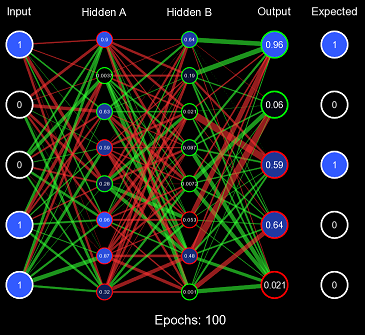
setting everything to zero! Let us illustrate this scheme graphically; we will create a three-layer network with sigmoid activation functions that learns to count in
binary. We will do this by feeding it a five binary digit number (0-31) and expecting it to predict that number plus one. For example: when fed the input 1 0 0 1 1 [19] the
expected output is 1 0 1 0 0 [20].
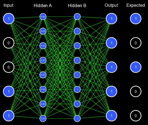
The network weights are represented by the lines; if they are green, it is a positive connection; if it is red, it is a negative connection. The thicker the line, the stronger the connection. For now, all the weights are initialized to one, so they are all equal. Biases are also represented by the outlines around the circle, if it is white, there is no bias, if it is green, there is a positive bias, and if it is red, there is a negative bias.
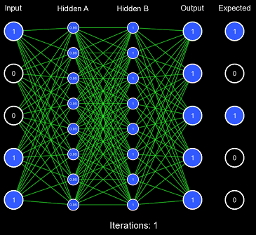
Now we are going to attempt to train this network; however, instead of training it on the set of all binary numbers, let us just attempt to train it to understand this single situation.
We will do this by getting the network to predict using the input 1 0 0 1 1, then using 1 0 1 0 0 as the expected output, applying standard backpropagation in
order to update the weights and biases. Let us apply this algorithm until the model accurately predicts the output for this situation. We will also use a quite high learning rate of 1.0
for these tests, as that should allow the network to train on this particular input VERY quickly.
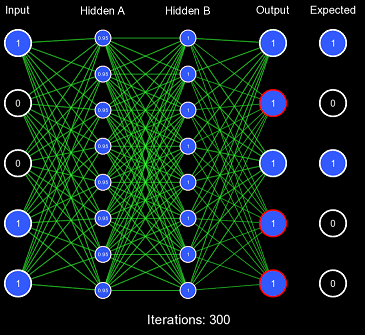
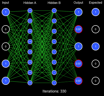
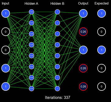
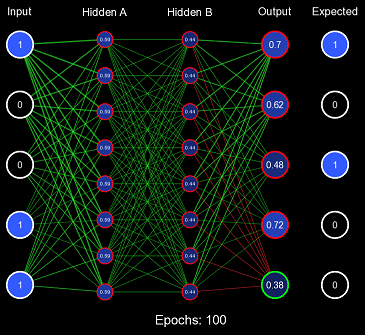
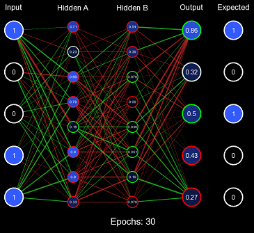
Despite our very large learning rate, it still took exactly 337 iterations for the network to finally predict correctly. This is FAR too slow to be acceptable performance, as this should've been accomplished in 1 or 2 iterations. This also demonstrates the first problem with this kind of initialization scheme: for some activation functions, predicting too extreme values produces a low derivative, which results in slow learning. You'll notice that the vast majority of the actual weight adjustments occur in the last few iterations; this is because, in the first iterations, the derivative is far too low, causing incredibly low gradients. Once the network has been slightly adjusted such that the derivatives become larger, more change can occur.
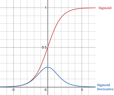
In this network, we are using the sigmoid activation function for every layer. The sigmoid function softly clamps the given value into the range (0, 1). Its formula and derivative is:
\(f(x) = \frac{1}{1 + e^{-x}}\)
\(f'(x) = f(x) * (1 - f(x))\)
Sigmoid is a very useful function; however, it can cause vanishing gradients in some situations, one of those situations we just saw. When the sigmoid function is pushed to its extremes, the derivative of the function is low at that point and results in lower gradients and slower learning.
So the first problem with the all 1s initialization scheme was it pushed clamping activation functions to their extremes, causing low derivatives and a vanishing gradient. Non-clamping activation functions (such as ReLU) don't have this problem; instead, they can suffer from exploding gradients because their value is uncapped. Now, let us view the second problem with this example by training on the entire 0-31 binary number dataset. We will define one epoch as performing the gradient descent algorithm once on each item in the dataset. Note: the order in which the dataset was iterated is random (this is because it increases convergence).
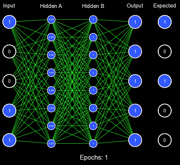
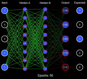
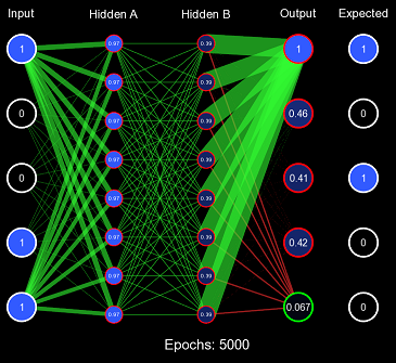
Obviously, the model is not converging; in fact, it never got more than 6/32 correct predictions on any epoch. This is the second problem with this initialization scheme: when the weights are too similar, the model has trouble creating useful decision boundaries. However, this is a gross exaggeration of the problem, as even a small amount of variance will quickly cascade into proper learning.
Doing it Right
Given the two problems discussed, let us attempt to think of possible solutions to them. In order to reduce the activation functions being pushed to their extremes, we can set the weights such that the starting activation will never be too high or too low (i.e., the magnitude of the nodes should remain low, but not too low or else no learning will occur). However, setting all of our weights to some pre-computed ideal value for the given activation function would not allow the model to create useful decision boundaries; therefore we should incorporate some kind of pseudo-randomness into our initialization scheme.
Xavier Initialization (named after one of the authors of the paper that pioneered the technique) addresses both of these concerns. There are many different adaptations, interpretations, and modifications of Xavier Initialization; we will only discuss the two mentioned in the paper: Standard Xavier Initialization and Normalized Xavier Initialization. The algorithm for Standard Xavier Initialization is to initialize all of your weights to be from a uniform distribution with the range being \((-\frac{1}{\sqrt{x}}, \frac{1}{\sqrt{x}})\) where \(x\) is the number of input nodes for the given layer (also known as fan-out; fan-in is the amount of output nodes for the given layer). Implemented in pseudo-code:
float bound = 1.0f / sqrt(inputCount);
for (int weightIdx = 0; weightIdx < inputCount * outputCount; weightIdx++)
{
    weights[weightIdx] = random.uniformDistribution(-bound, bound);
}
This solves both problems, the range of the distribution is designed to maintain the variance of the values when forward propagating, and it is also randomized so it can quickly produce valuable decision boundaries. Let us test this initialization scheme using the same method before, but instead of All 1s Initialization, we will use Standard Xavier Initialization.
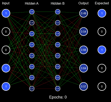
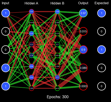
Evidently, this is far improved from All 1s Initialization, the values of the nodes are initially kept to a small value where the derivative at that point is still a large enough number for efficient learning, and the values are randomized effectively so that decision boundaries can form. However, Standard Xavier Initialization was only designed to regulate the variance when feeding forward. Backpropagation is just as valuable to a model as forward-propagation. For this purpose, there is Normalized Xavier Initialization, where the algorithm is incredibly similar to Standard Xavier Initialization; however, it attempts to regulate both the variance moving forward and the variance moving backward. It also utilizes a uniform distribution ; but with a range of \((-\frac{\sqrt{6}}{\sqrt{x + y}}, \frac{\sqrt{6}}{\sqrt{x + y}})\) where \(x\) is the number of input nodes and \(y\) is the number of output nodes.
Uniform distributions are not the only method of applying randomness; a common approach is using a normal distribution. One approach that uses a normal distribution is Kaiming Initialization (we will address a slightly simplified version, for more information, see this paper). Kaiming Initialization uses a standard deviation with a mean of \(0\) and a standard deviation of \(\sqrt{\frac{2}{x}}\) where \(x\) can either be the number of input nodes, or the number of output nodes (depends on if you choose to preserve the magnitude while forward-propagating [using input node count/fan-out], or while backpropagating [using output node count/fan-in]).
These initialization schemes are both among the leading modern approaches to weight initialization. They are typically used for different purposes; Xavier is generally used for networks with sigmoidal activation functions (Sigmoid, TanH, etc.), whereas Kaiming is generally used for large networks (20+ layers) with a lot of linear activation functions (ReLU, LeakyReLU, etc.).
What can be improved?
Variance Preservation v.s. Magnitude Preservation
Xavier and Kaiming initialization have one main feature in common; they are designed to preserve the variance of the values while being propagated. This means that when backpropagating through the network, the magnitude of the gradients may differ from layer to layer, but the variance (square of the standard deviation) would stay consistent. Instead of preserving the variance of the gradients while backpropagating, wouldn't it make more sense to preserve the magnitude of the gradients? If the magnitude of the gradients were conserved while backpropagating, the gradients of the layers earlier in the network would be roughly equivalent to the layers closer to the output, possibly allowing for more even training. This is all speculation; the only thing left to do is to test our theory.
Let us start by testing how well Xavier preserves the magnitude of its input. We can test this by writing a Python program to emulate a Xavier initialization many MANY times for many different sized layers, then evaluating the average magnitude of the outputs. The Python code for it is:
import random
import math


def test_uniform_magnitude_preservation(input_count, bound):
    """ Simulates propagating with an input of all 1s, with weights initialized using a uniform distribution
    then returns the absolute value of the output."""
    value = 0.0

    for _ in range(input_count):
        value += random.uniform(-bound, bound)  # assume every input is 1, therefore we can just add the weight

    return abs(value)


iterations = 1000000
layer_sizes = [1, 5, 25, 100, 300, 1000]

for size in layer_sizes:
    xavier_bound = 1.0 / math.sqrt(size)

    total = 0.0
    for i in range(iterations):
        total += test_uniform_magnitude_preservation(size, xavier_bound)

    print("Layer size: " + str(size) + "   |   magnitude: " + str(total / iterations))
The code produced this output:
Layer size: 1   |   magnitude: 0.500474810495207
Layer size: 5   |   magnitude: 0.4658366066117104
Layer size: 25   |   magnitude: 0.4617913077193642
Layer size: 100   |   magnitude: 0.4611953525250335
Layer size: 300   |   magnitude: 0.4603023799913436
Layer size: 1000   |   magnitude: 0.4605755033078747
Interesting, so it appears that at least experimentally, Xavier Initialization does not preserve magnitude. Now let us try to recreate these values theoretically by finding a formula for how much magnitude was preserved given the layer size.
Standard Letkeman Initialization
Currently, we calculate the magnitude preservation by doing a sum of uniform distributions several times. Luckily, there is a formula for exactly this, it is called the Irwin-Hall Distribution, it creates a probability curve for the sum of \(n\) uniform distributions that each have the range [0, 1]. It's formula is:
\(f(x)=\frac{n}{2(n-1)!}\sum_{k=0}^{n}(-1)^{k}{{n}\choose{k}}(x-k)^{n-1}{\operatorname{sgn}}(x-k)\)
Despite being a slightly difficult formula to work with, this is great! However, Xavier weight initializations are not in the range of \([0, 1]\) therefore we need to manually tune this function slightly to emulate our uniform distributions being in the range of \((-\frac{1}{\sqrt{n}}, \frac{1}{\sqrt{n}})\).
\(g(x)=\frac{f(\frac{{x}\sqrt{n}}{2}+\frac{n}{2})}{{2}\sqrt{n}}\)
This gives us the probability of each weight value, now we just need to multiply by the absolute value of \(x\) to get our actual expected value from the weight.
\(h(x)=g(x)|x|\)
Finally, we can intergrate from \((-\sqrt{n}, \sqrt{n})\) (the minimum and maximum possible ranges of our sum of Xavier uniform distributions) to get our final expected magnitude preservation.
\(\int_{-\sqrt{n}}^{\sqrt{n}}h(x)dx\)
Written out in its entirety, we get this behemoth:
\(\int_{-\sqrt{n}}^{\sqrt{n}}\frac{\frac{n}{2(n-1)!}\sum_{k=0}^{n}(-1)^{k}{{n}\choose{k}}(\frac{{x}\sqrt{n}}{2}+\frac{n}{2}-k)^{n-1}{\operatorname{sgn}}(\frac{{x}\sqrt{n}}{2}+\frac{n}{2}-k)}{{2}\sqrt{n}}|x|dx\)
This is quite a beast to calculate whenever you need to initialize a layer (remember you would need to re-integrate this and substitute \(n\) with the amount of input nodes. To solve this problem, we can use an approximation function instead:
def approximate(n):
    # Hardcode the first few values, then use an approximation function after that
    if n == 1:
        return 0.5
    if n == 2:
        return 0.471404520791
    if n == 3:
        return 0.469097093716
    a = 0.039
    return (0.5 - a) + ((1.0 / math.sqrt(2.0 * n - 1.0)) ** 2) * a
Now, if we were to take our Xavier bounds and divide by this approximated integral, we should get a magnitude very close to 1. Let us test that:
Layer size: 1   |   magnitude: 0.9997531021498397
Layer size: 5   |   magnitude: 1.0006271684273118
Layer size: 25   |   magnitude: 0.9997050090618478
Layer size: 100   |   magnitude: 0.9996631602474665
Layer size: 300   |   magnitude: 1.0000115563283445
Layer size: 1000   |   magnitude: 1.0003759838261814
Therefore, if we initialize our weights using a uniform distribution with the range \((-\frac{\frac{1}{\sqrt{x}}}{\int_{-\sqrt{n}}^{\sqrt{n}}\frac{\frac{n}{2(n-1)!}\sum_{k=0}^{n}(-1)^{k}{{n}\choose{k}}(\frac{{x}\sqrt{n}}{2}+\frac{n}{2}-k)^{n-1}{\operatorname{sgn}}(\frac{{x}\sqrt{n}}{2}+\frac{n}{2}-k)}{{2}\sqrt{n}}|x|dx}, \frac{\frac{1}{\sqrt{x}}}{\int_{-\sqrt{n}}^{\sqrt{n}}\frac{\frac{n}{2(n-1)!}\sum_{k=0}^{n}(-1)^{k}{{n}\choose{k}}(\frac{{x}\sqrt{n}}{2}+\frac{n}{2}-k)^{n-1}{\operatorname{sgn}}(\frac{{x}\sqrt{n}}{2}+\frac{n}{2}-k)}{{2}\sqrt{n}}|x|dx})\) (where \(n\) is the number of nodes in the input layer) the magnitude should, on average, be the same as the magnitude of the inputs. For the sake of brevity, I'm going to refer to this as Standard Letkeman Initialization.
Normalized Letkeman Initialization
There is a problem with Standard Letkeman Initialization; it only ensures that the magnitude is maintained during the forward pass but does nothing for backpropagation. Just like how Standard Xavier Initialization has its normalized counter-part that is designed to regulate both the forward pass and the backward pass. However, this introduces some complications; the only situation in which the magnitude is perfectly preserved in both the forward pass and the backward pass is if the number of input and output nodes for that layer is equal. If the numbers are unequal, the magnitude is not going to be perfectly preserved in at least one of the directions; our solution to this is just to make the average magnitude preservation across all nodes one (for both the forward and backward pass); this will require changing our experimental testing program slightly:
import random
import math


def test_normalized_uniform_magnitude_preservation(input_count, output_count, bound):
    """ Simulates propagating with an input of all 1s, with weights initialized using a uniform distribution
    then returns the absolute value of the output for both forward and backward propagation."""

    # for this version of the function we'll have to simulate the entirety of the forward and backward passes
    # as well as creating the weight matrix
    weights = [[random.uniform(-bound, bound) for __ in range(output_count)] for _ in range(input_count)]

    total_forward_magnitudes = 0.0
    for i in range(input_count):
        value = 0.0
        for o in range(output_count):
            value += weights[i][o]  # assume every input is 1, therefore we can just add the weight
        total_forward_magnitudes += abs(value)

    total_backward_magnitudes = 0.0
    for o in range(output_count):
        value = 0.0
        for i in range(input_count):
            value += weights[i][o]  # assume every input is 1, therefore we can just add the weight
        total_backward_magnitudes += abs(value)

    return total_forward_magnitudes / float(output_count), total_backward_magnitudes / float(input_count), \
            (total_forward_magnitudes + total_backward_magnitudes) / float(input_count + output_count)


iterations = 5000
layer_sizes = [(1, 1), (5, 5), (100, 1), (15, 25), (10, 100), (100, 50), (100, 300), (1000, 10), (1, 10000), (3, 10000)]

for size in layer_sizes:
    normalized_xavier_bound = math.sqrt(6.0) / math.sqrt(size[0] + size[1])

    forward_total = 0.0
    backward_total = 0.0
    avg_total = 0.0
    for i in range(iterations):
        forward, backward, avg = test_normalized_uniform_magnitude_preservation(size[0], size[1],
                                                                                normalized_xavier_bound)
        forward_total += forward
        backward_total += backward
        avg_total += avg

    print("Layer size: " + str(size) +
            "   |   forward magnitude: " + str(forward_total / iterations) +
            "   |   backward magnitude: " + str(backward_total / iterations) +
            "   |   avg magnitude: " + str(avg_total / iterations))
Which when ran produced these results:
Layer size: (1, 1)   |   forward magnitude: 0.8594973435645746   |   backward magnitude: 0.8594973435645746   |   avg magnitude: 0.8594973435645746
Layer size: (5, 5)   |   forward magnitude: 0.8084311839378276   |   backward magnitude: 0.8045734522931961   |   avg magnitude: 0.806502318115512
Layer size: (100, 1)   |   forward magnitude: 12.187413775506647   |   backward magnitude: 0.011053896083235643   |   avg magnitude: 0.1316119146913889
Layer size: (15, 25)   |   forward magnitude: 0.5368980806669289   |   backward magnitude: 1.1514005259906934   |   avg magnitude: 0.7673364976633413
Layer size: (10, 100)   |   forward magnitude: 0.1077280335302238   |   backward magnitude: 3.4205235980572755   |   avg magnitude: 0.4088912666690458
Layer size: (100, 50)   |   forward magnitude: 1.3046534263608478   |   backward magnitude: 0.46020072148131086   |   avg magnitude: 0.7416849564411578
Layer size: (100, 300)   |   forward magnitude: 0.3257606846562078   |   backward magnitude: 1.6939843417948686   |   avg magnitude: 0.6678165989408731
Layer size: (1000, 10)   |   forward magnitude: 11.277801840070467   |   backward magnitude: 0.011307052186118244   |   avg magnitude: 0.1228565055315076
Layer size: (1, 10000)   |   forward magnitude: 0.00011277174801493292   |   backward magnitude: 122.47346786077979   |   avg magnitude: 0.01235888264582831
Layer size: (3, 10000)   |   forward magnitude: 0.0003375413496494392   |   backward magnitude: 66.31341829144523   |   avg magnitude: 0.020225499187326784
Just like what we did with Standard Letkeman Initialization, let us try to recreate these values theoretically by finding a formula for how much magnitude was preserved given the input layers size as \(n\) and the output layers size as \(m\). We can use the same Irwin-Hall distribution; however, we will need one distribution for the forward pass, and one for the backward pass.
\(f(x)=\frac{n}{2(n-1)!}\sum_{k=0}^{n}(-1)^{k}{{n}\choose{k}}(x-k)^{n-1}{\operatorname{sgn}}(x-k)\)
\(g(x)=\frac{m}{2(m-1)!}\sum_{k=0}^{m}(-1)^{k}{{m}\choose{k}}(x-k)^{m-1}{\operatorname{sgn}}(x-k)\)
Again, this represents the uniform distributions as having a range of \([0, 1]\), so we need functions to convert their range to Normalized Xavier ranges of \((-\frac{\sqrt{6}}{\sqrt{n+m}}, \frac{\sqrt{6}}{\sqrt{n+m}})\)
\(h(x)=\frac{f(\frac{{x}\sqrt{n+m}}{2\sqrt{6}}+\frac{n}{2})}{\frac{2n\sqrt{6}}{\sqrt{n+m}}}\)
\(l(x)=\frac{g(\frac{{x}\sqrt{n+m}}{2\sqrt{6}}+\frac{m}{2})}{\frac{2m\sqrt{6}}{\sqrt{n+m}}}\)
This gives us the probability of each weight value for the forward and backward passes, now we need to multiply by \(|x|\) to get our actual expected value from the weight.
\(u(x)=h(x)|x|\)
\(v(x)=l(x)|x|\)
Now we integrate from \((-\frac{n\sqrt{6}}{\sqrt{n+m}},\frac{n\sqrt{6}}{\sqrt{n+m}})\) for our forward pass, and \((-\frac{m\sqrt{6}}{\sqrt{n+m}},\frac{m\sqrt{6}}{\sqrt{n+m}})\) for our backward pass.
\(q=\int_{-\frac{n\sqrt{6}}{\sqrt{n+m}}}^{\frac{n\sqrt{6}}{\sqrt{n+m}}}u(x)dx\)
\(p=\int_{-\frac{m\sqrt{6}}{\sqrt{n+m}}}^{\frac{m\sqrt{6}}{\sqrt{n+m}}}v(x)dx\)
Finally, we can sum our results together for our final calculation.
\(\frac{nq+mp}{n+m}\)
Written as a whole (the faint of heart may want to avert their eyes away from this transgression against God and Man):
\(\frac{n\left(\int_{-\frac{n\sqrt{6}}{\sqrt{n+m}}}^{\frac{n\sqrt{6}}{\sqrt{n+m}}}\frac{\frac{n}{2\left(n-1\right)!}\sum_{k=0}^{n}\left(-1\right)^{k}{{n}\choose{k}}\left(\frac{x\sqrt{n+m}}{2\sqrt{6}}+\frac{n}{2}-k\right)^{\left(n-1\right)}\operatorname{sgn}\left(\frac{x\sqrt{n+m}}{2\sqrt{6}}+\frac{n}{2}-k\right)\left|x\right|}{\frac{2n\sqrt{6}}{\sqrt{n+m}}}dx\right)+m\left(\int_{-\frac{m\sqrt{6}}{\sqrt{n+m}}}^{\frac{m\sqrt{6}}{\sqrt{n+m}}}\frac{\frac{m}{2\left(m-1\right)!}\sum_{k=0}^{m}\left(-1\right)^{k}{{n}\choose{k}}\left(\frac{x\sqrt{n+m}}{2\sqrt{6}}+\frac{m}{2}-k\right)^{\left(m-1\right)}\operatorname{sgn}\left(\frac{x\sqrt{n+m}}{2\sqrt{6}}+\frac{m}{2}-k\right)\left|x\right|}{\frac{2m\sqrt{6}}{\sqrt{n+m}}}dx\right)}{n+m}\)
Again, it is incredibly expensive to compute this at run-time, so we can use an approximation function that utilizes our previous approximation function:
def approximate_a(n):
    a = 0.073
    return (0.866 - a) + (1.0 / math.sqrt(6.0 * n - 5.0)) * a

def approximate_b(n):
    b = -0.08
    return (1.0 - b) + (1.0 / math.sqrt(6.0 * n - 5.0)) * b

def approximate_c(n):
    return 1 / math.sqrt(0.5 * n + 0.5)

def approximate_normalized(n, m):
    highest = n if n >= m else m
    lowest = m if n >= m else n
    return approximate_a(lowest) * approximate_b(highest - lowest + 1) * approximate_c(highest / lowest)
Now we take the Normalized Xavier bounds, divide by it using this approximation function. When we run this we get this output:
Layer size: (1, 1)   |   forward magnitude: 0.9943010700551295   |   backward magnitude: 0.9943010700551295   |   avg magnitude: 0.9943010700551295
Layer size: (5, 5)   |   forward magnitude: 0.9993559541424449   |   backward magnitude: 1.0016561989451123   |   avg magnitude: 1.0005060765437785
Layer size: (100, 1)   |   forward magnitude: 92.90548094688566   |   backward magnitude: 0.08605654405489507   |   avg magnitude: 1.0050607460631158
Layer size: (15, 25)   |   forward magnitude: 0.7219516088992118   |   backward magnitude: 1.552360250077088   |   avg magnitude: 1.0333548493409184
Layer size: (10, 100)   |   forward magnitude: 0.29088207337482874   |   backward magnitude: 9.277565035000634   |   avg magnitude: 1.1078532517044446
Layer size: (100, 50)   |   forward magnitude: 1.8668152727502358   |   backward magnitude: 0.657427648552596   |   avg magnitude: 1.0605568566184786
Layer size: (100, 300)   |   forward magnitude: 0.5372220506522588   |   backward magnitude: 2.790470951744516   |   avg magnitude: 1.1005342759253183
Layer size: (1000, 10)   |   forward magnitude: 92.54224171674791   |   backward magnitude: 0.09236415107640739   |   avg magnitude: 1.0077094735088017
Layer size: (1, 10000)   |   forward magnitude: 0.008441322648025064   |   backward magnitude: 9262.953664512319   |   avg magnitude: 0.93464322477678
Layer size: (3, 10000)   |   forward magnitude: 0.015693092438484952   |   backward magnitude: 3084.4314192973225   |   avg magnitude: 0.9407402961388404
Therefore, if we initialize our weights using a uniform distribution with the range: \(\begin{split}(-\frac{\frac{\sqrt{6}}{\sqrt{n+m}}}{\frac{n\left(\int_{-\frac{n\sqrt{6}}{\sqrt{n+m}}}^{\frac{n\sqrt{6}}{\sqrt{n+m}}}\frac{\frac{n}{2\left(n-1\right)!}\sum_{k=0}^{n}\left(-1\right)^{k}{{n}\choose{k}}\left(\frac{x\sqrt{n+m}}{2\sqrt{6}}+\frac{n}{2}-k\right)^{\left(n-1\right)}\operatorname{sgn}\left(\frac{x\sqrt{n+m}}{2\sqrt{6}}+\frac{n}{2}-k\right)\left|x\right|}{\frac{2n\sqrt{6}}{\sqrt{n+m}}}dx\right)+m\left(\int_{-\frac{m\sqrt{6}}{\sqrt{n+m}}}^{\frac{m\sqrt{6}}{\sqrt{n+m}}}\frac{\frac{m}{2\left(m-1\right)!}\sum_{k=0}^{m}\left(-1\right)^{k}{{n}\choose{k}}\left(\frac{x\sqrt{n+m}}{2\sqrt{6}}+\frac{m}{2}-k\right)^{\left(m-1\right)}\operatorname{sgn}\left(\frac{x\sqrt{n+m}}{2\sqrt{6}}+\frac{m}{2}-k\right)\left|x\right|}{\frac{2m\sqrt{6}}{\sqrt{n+m}}}dx\right)}{n+m}},\\ \frac{\frac{\sqrt{6}}{\sqrt{n+m}}}{\frac{n\left(\int_{-\frac{n\sqrt{6}}{\sqrt{n+m}}}^{\frac{n\sqrt{6}}{\sqrt{n+m}}}\frac{\frac{n}{2\left(n-1\right)!}\sum_{k=0}^{n}\left(-1\right)^{k}{{n}\choose{k}}\left(\frac{x\sqrt{n+m}}{2\sqrt{6}}+\frac{n}{2}-k\right)^{\left(n-1\right)}\operatorname{sgn}\left(\frac{x\sqrt{n+m}}{2\sqrt{6}}+\frac{n}{2}-k\right)\left|x\right|}{\frac{2n\sqrt{6}}{\sqrt{n+m}}}dx\right)+m\left(\int_{-\frac{m\sqrt{6}}{\sqrt{n+m}}}^{\frac{m\sqrt{6}}{\sqrt{n+m}}}\frac{\frac{m}{2\left(m-1\right)!}\sum_{k=0}^{m}\left(-1\right)^{k}{{n}\choose{k}}\left(\frac{x\sqrt{n+m}}{2\sqrt{6}}+\frac{m}{2}-k\right)^{\left(m-1\right)}\operatorname{sgn}\left(\frac{x\sqrt{n+m}}{2\sqrt{6}}+\frac{m}{2}-k\right)\left|x\right|}{\frac{2m\sqrt{6}}{\sqrt{n+m}}}dx\right)}{n+m}})\end{split}\)
That should make the average magnitude preservation of both the forward and backward pass to be equal to 1. I am going to refer to this as Normalized Letkeman Initialization.
Usage
We are also going to do one thing differently compared to Xavier and Kaiming; there are some situations in which the number of nodes in the input layer isn't necessarily the number of active nodes in that layer. Namely when our input is either a one-hot vector or the product of a softmax activation. As a refresher, a one-hot vector is when you have a vector of all 0s except for one entry which is a 1, and a softmax activation clamps the total activated output to 1 according to this formula: \(f(x)_{i} = \frac{e^{x}}{\sum_{j=0}^{n}e^{j}}\) (essentially set each element of the vector to \(e\) raised to that element, then divide by the sum of all elements in the vector). In both of these situations, the guaranteed magnitude of the layer is 1; therefore, we can treat the entire layer as a single input node. As the magnitude of that layer is always 1, the actual size of that layer is irrelevant and we can always treat it as 1.
This is something that Xavier and Kaiming don't account for, and we will see in the following results section that this can have a substantial impact on the speed of our learning. I will refer to this method of determining the input nodes as the Active Node Method. As we will see in the results section, adding this slight change can have drastic improvements compared to the traditional fan-in method.
Results
Overall Results
I compared these five initialization methods (Standard Xavier, Normalized Xavier, Standard Letkeman, Normalize Letkeman, and Kaiming) against each other using four different networks. For each network and initialization method, I ran the simulation five different times using the seeds 1-5, just to get an average. I also ensured that the randomness was consistent (for all the initialization methods that utilized a uniform distribution, the distribution always gave a similar number for each weight, the only thing that changed was the initialization method modifying the range of the weights). I then created graphs of their training loss versus epochs which can be used to compare how efficiently the networks trained.
The four networks I used were: the binary counting network presented earlier in this article (the only difference being a learning rate of 0.1 instead), a convolutional network for the MNIST digit dataset, a large dense network that utilizes sigmoid activation functions for the MNIST digit dataset, and a recurrent neural network trained to replicate Shakespeare's Hamlet. These networks were not selected because they are the best at accomplishing their given task (they all perform to varying degrees of success), but because they represent a wide variety of different networks and tasks. All the data can be downloaded here.
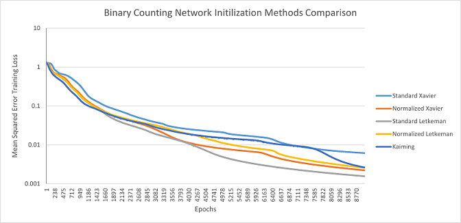
Binary Counting Network: Standard Letkeman seems to have a noticeable advantage for this network; something to note is that on the 5th seed, Kaiming slowed down quite considerably closer to the end of the training, causing its average to fall noticeably behind, despite Kaiming performing quite comparable to Standard Letkeman on the other seeds.
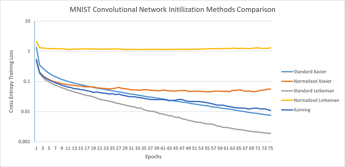
MNIST Convolutional Network: Standard Letkeman appears to train significantly more effectively than the other initilization algorithms; much like in the Binary Counting Network, Kaiming started training incredibly slow on the 3rd seed, which brought it's average much lower. Normalized Letkeman failed to converge in 2/5 seeds for this network architecture, and trained incredibly slow on the other seeds. This is most likely due to the later layers in the network having far fewer nodes than the previous, causing those layers' activation values to skyrocket, causing a vanishing gradient. Standard Xavier's average loss at the end of the 75 epochs was 0.007568, Standard Letkeman was able to surpass that in 43 epochs; meaning that Standard Letkeman trained at 1.744x the speed of Standard Xavier (the next fastest method).
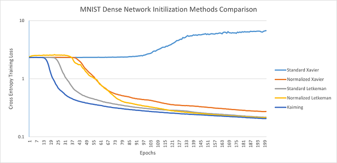
MNIST Dense Network: Kaiming was able to escape the plateau first, followed by Standard Letkeman, then Kaiming and both forms of Letkeman approached roughly the same values, with Kaiming having a very slight lead. Standard Xavier was unable to converge in this architecture, likely due to weights being initilized too low, resulting in the weights having little effect near the end of the network, causing it to be unable to train.
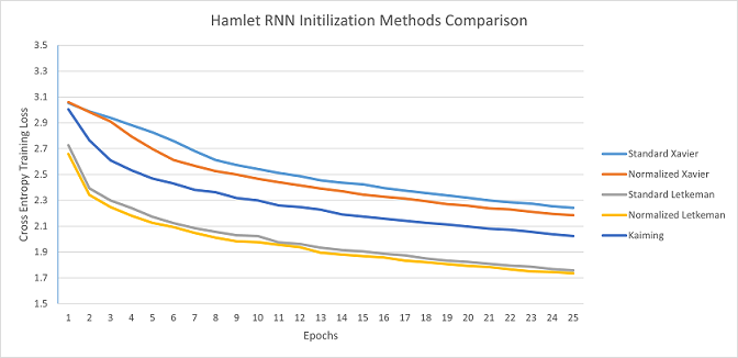
Hamlet RNN: Standard and Normalized Letkeman clearly trained far faster than any of the alternatives, with Normalized Letkeman being slightly faster than Standard letkeman. It is also worthy to note that the data for these tests was incredibly regular and consistent, with minimal irregularities between the seeds. Kaiming's average loss at the end of the 25 epochs was 2.024412, Standard Letkeman surpassed that loss in 10 epochs, while Normalized Letkeman only took 8 epochs to surpass Kaiming; meaning that Standard Letkeman trained at 2.5x the speed of Kaiming, while Normalized Letkeman trained at 3.125x speed (although as you will see in the next section, the majority of that change is from Letkeman methods utilizing the active node method of counting input nodes, which is something that other methods can utilize with only small adjustments).
Active Node Method
The only one of these networks to utilize the active node method was the RNN used to predict Shakespeare's Hamlet, it utilized a one-hot vector of all the possible characters in the input layer (ex. if the current character was an 'a', then only the node corresponding to 'a' would be set to 1, all others would be 0). I ran two sets of tests for this, one test where the Xavier and Kaiming initialization methods utilized the Active Node Method (ANM), and another test where they didn't; I then compared those to Letkeman methods (which always use ANM).
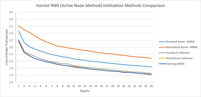
As you can see with the Active Node Method, Kaiming and Letkeman train at nearly the exact same rate (in fact, Kaiming is very slightly faster). It is quite evident that using the ANM greatly improves training speed.
Conclusion
Given the results of the tests, Standard Letkeman initialization appears to be a more consistent and effective method for initializing weights compared to Xavier and Kaiming; in some cases even cutting training time by 68%. However, these tests were not exhaustive and are not indicative of all possible machine learning models you may want to utilize. As such, it is important to do your own tests and judge which method performs best for your network architecture. However, testing has shown that Standard Letkeman initialization is an effective initialization algorithm for most machine learning models.